
Modelling tabular data with CatBoost and NODE
CatBoost from Yandex, a Russian online search company, is fast and easy to use, but recently researchers from the same company released a new neural network based package, NODE, that they claim outperforms CatBoost and all other gradient boosting methods. Can this be true? Let’s find out how to use both CatBoost and NODE!
Who is this blog post for?
Although I wrote this blog post for anyone who is interested in machine learning and in particular tabular data, it is helpful if you are familiar with Python and the scikit-learn library if you want to follow along with the code. If you aren’t, hopefully you will find the theoretical and conceptual parts interesting anyway!
CatBoost introduction
CatBoost is my go-to package for modelling tabular data. It is an implementation of gradient boosted decision trees with a few tweaks that make it slightly different from e.g. xgboost or LightGBM. It works for both classification and regression problems.
Some nice things about CatBoost:
- It handles categorical features (get it?) out of the box, so you don’t need to worry about how to encode them.
- It typically requires very little parameter tuning.
- It avoids certain subtle types of data leakage that other methods may suffer from.
- It is fast, and can be run on GPU if you want it to go even faster.
These factors make CatBoost, for me, a no-brainer as the first thing to reach for when I need to analyze a new tabular dataset.
Technical details of CatBoost
Skip this section if you just want to use CatBoost!
On a more technical level, there are some interesting things about how CatBoost is implemented. I highly recommend the paper Catboost: unbiased boosting with categorical features if you are interested in the details. I just want to highlight two things.
- In the paper, the authors show that standard gradient boosting algorithms are affected by subtle types of data leakage which result from the way that the models are iteratively fitted. In a similar manner, the most effective ways to encode categorical features numerically (like target encoding) are prone to data leakage and overfitting. To avoid this leakage, CatBoost introduces an artificial timeline according to which the training examples arrive, so that only “previously seen” examples can be used when calculating statistics.
- CatBoost actually doesn’t use regular decision trees, but oblivious decision trees. These are trees where, at each level of the tree, the same feature and the same splitting criterion is used everywhere! This sounds weird, but has some nice properties. Let’s look at what is meant by this.


Left: Regular decision tree. Any feature or split point can be present at each level. Right: Oblivious decision tree. Each level has the same splits.
In a normal decision tree, feature to split on and the cutoff value both depend on what path you have taken so far in the tree. This makes sense, because we can use the information we already have to decide the most informative next question (like in the “20 questions” game). With oblivious decision trees, the history doesn’t matter; we pose the same question no matter what. The trees are called “oblivious” because they keep “forgetting” what has happened before.
Why is this useful? One nice property of oblivious decision trees is that an example can be classified or scored really quickly – it is always the same N binary questions that are posed (where N is the depth of the tree). This can easily be done in parallel for many examples. That is one reason why CatBoost is fast. Another thing to keep in mind is that we are dealing with a tree ensemble here. As a stand-alone algorithm, the oblivious decision tree might not work so well, but the idea of tree ensembles is that a coalition of weak learners often works well because errors and biases are “washed out”. Normally, the weak learner is a standard decision tree, and here it is something even weaker, namely the oblivious decision tree. The CatBoost authors argue that this particular weak base learner works well for generalization.
Installing CatBoost
Although installing CatBoost should be a simple matter of typing
pip install catboost
I’ve sometimes encountered problems with that when on a Mac. On Linux systems such as the Ubuntu system I am typing on now, or on Google Colaboratory, it should “just work”. If you keep having problems installing it, consider using a Docker image, e.g.
docker pull yandex/tutorial-catboost-clickhouse
docker run -it yandex/tutorial-catboost-clickhouse
Using CatBoost on a dataset
Link to Colab notebook with code
Let’s have a look at how to use CatBoost on a tabular dataset. We start by downloading a lightly preprocessed version of the Adult/Census Income dataset which is, in the following, assumed to be located in datasets/adult.csv. I chose this dataset because it has a mix of categorical and numerical features, a nice manageable size in the tens of thousands of examples and not too many features. It is often used to exemplify algorithms, for instance in Google’s What-If Tool and many other places.
The adult census dataset has the columns ‘age’, ‘workclass’, ‘education’, ‘education-num’, ‘marital-status’, ‘occupation’, ‘relationship’, ‘race’, ‘sex’, ‘capital-gain’, ‘capital-loss’, ‘hours-per-week’, ‘native-country’, and ‘<=50K‘. The task is to predict the value of the last column, ‘<=50K’, which indicates if the person in question earns 50,000 USD or less per year (the dataset is from 1994). We regard the following features as categorical rather than numerical: ‘workclass’, ‘education’, ‘marital-status’, ‘occupation’, ‘relationship’, ‘race’, ‘sex’, ‘native-country’.
The code is pretty similar to scikit-learn except for the Pool datatype that CatBoost uses to bundle feature and target values for a dataset while keeping them conceptually separate. (I have to admit I don’t really know why Pool is there – I just use it, and it seems to work fine.)
The code is available on Colab, but I will copy it here for reference. CatBoost needs to know which features are categorical and will then handle them automatically. In this code snippet, I also use 5-fold (stratified) cross-validation to estimate the prediction accuracy.
from catboost import CatBoostClassifier, Pool
from hyperopt import fmin, hp, tpe
import pandas as pd
from sklearn.model_selection import StratifiedKFold

df = pd.read_csv("https://docs.google.com/uc?" +
                 "id=10eFO2rVlsQBUffn0b7UCAp28n0mkLCy7&" +
                 "export=download")
labels = df.pop('<=50K')

categorical_names = ['workclass', 'education', 'marital-status',
                     'occupation', 'relationship', 'race',
                     'sex', 'native-country']
categoricals = [df.columns.get_loc(i) for i in categorical_names]

nfolds = 5
skf = StratifiedKFold(n_splits=nfolds, shuffle=True)
acc = []

for train_index, test_index in skf.split(df, labels):
  X_train, X_test = df.iloc[train_index].copy(), \
                    df.iloc[test_index].copy()
  y_train, y_test = labels.iloc[train_index], \
                    labels.iloc[test_index]
  train_pool = Pool(X_train, y_train, cat_features = categoricals)
  test_pool = Pool(X_test, y_test, cat_features = categoricals)
  model = CatBoostClassifier(iterations=100,
                             depth=8,
                             learning_rate=1,
                             loss_function='MultiClass')
  model.fit(train_pool)
  predictions = model.predict(test_pool)
  accuracy = sum(predictions.squeeze() == y_test) / len(predictions)
  acc.append(accuracy)

mean_acc = sum(acc) / nfolds
print(f'Mean accuracy based on {nfolds} folds: {mean_acc:.3f}')
print(acc)
What we tend to get from running this (CatBoost without hyperparameter optimization) is a mean accuracy between 85% and 86%. In my last run, I got about 85.7%.
If we want to try to optimize the hyperparameters, we can use hyperopt (if you don’t have it, install it with pip install hyperopt). In order to use it, you need to define a function that hyperopt tries to minimize. We will just try to optimize the accuracy here. Perhaps it would be better to optimize e.g. log loss, but that is left as an exercise to the reader 😉
The main parameters to optimize are probably the number of iterations, the learning rate, and the tree depth. There are also many other parameters related to over-fitting, for instance early stopping rounds and so on. Feel free to explore on your own!
# Optimize between 10 and 1000 iterations and depth between 2 and 12

search_space = {'iterations': hp.quniform('iterations', 10, 1000, 10),
                'depth': hp.quniform('depth', 2, 12, 1),
                'lr': hp.uniform('lr', 0.01, 1)
               }

def opt_fn(search_space):

  nfolds = 5
  skf = StratifiedKFold(n_splits=nfolds, shuffle=True)
  acc = []

  for train_index, test_index in skf.split(df, labels):
    X_train, X_test = df.iloc[train_index].copy(), \
                      df.iloc[test_index].copy()
    y_train, y_test = labels.iloc[train_index], \
                      labels.iloc[test_index]
    train_pool = Pool(X_train, y_train, cat_features = categoricals)
    test_pool = Pool(X_test, y_test, cat_features = categoricals)

    model = CatBoostClassifier(iterations=search_space['iterations'],
                             depth=search_space['depth'],
                             learning_rate=search_space['lr'],
                             loss_function='MultiClass',
                             od_type='Iter')

    model.fit(train_pool, logging_level='Silent')
    predictions = model.predict(test_pool)
    accuracy = sum(predictions.squeeze() == y_test) / len(predictions)
    acc.append(accuracy)

  mean_acc = sum(acc) / nfolds
  return -1*mean_acc

best = fmin(fn=opt_fn,
            space=search_space,
            algo=tpe.suggest,
            max_evals=100)
When I last ran this code, it took over 5 hours but resulted in a mean accuracy of 87.3%, which is on par with the best results I got when trying the Auger.ai AutoML platform.
Sanity check: logistic regression
At this point we should ask ourselves if these fancy new-fangled methods are really needed. How would a good old logistic regression perform out of the box and after hyperparameter optimization?
I’ll omit reproducing the code here for brevity’s sake, but it is available in the same Colab notebook as before. One detail with the logistic regression implementation is that it doesn’t handle categorical variables out of the box like CatBoost does, so I decided to code them using target encoding, specifically leave-one-out target encoding, which is the approach taken in NODE and a fairly close though not identical analogue of what happens in CatBoost.
Long story short, untuned logistic regression with this type of encoding yields around 80% accuracy, and around 81% (80.7% in my latest run) after hyperparameter tuning. Here, an interestin alternative is to try automated preprocessing libraries such as vtreat and Automunge, but I will save those for an upcoming blog post!
Taking stock
What do we have so far, before trying NODE?
- Logistic regression, untuned: 80.0%
- Logistic regression, tuned: 80.7%
- CatBoost, untuned: 85.7%
- CatBoost, tuned: 87.2%
NODE: Neural Oblivious Decision Ensembles
A recent manuscript from Yandex researchers describes an interesting neural network version of CatBoost, or at least a neural network take on oblivious decision tree ensembles (see the technical section above if you want to remind yourself what “oblivious” means here.) This architecture, called NODE, can be used for either classification or regression.
One of the claims from the abstract reads: “With an extensive experimental comparison to the leading GBDT packages on a large number of tabular datasets, we demonstrate the advantage of the proposed NODE architecture, which outperforms the competitors on most of the tasks.” This naturally piqued my interest. Could this tool be better than CatBoost?
How does NODE work?
You should go to the paper for the full story, but some relevant details are:
- The entmax activation function is used as a soft version of a split in a regular decision tree. As the paper puts it, “The entmax is capable to produce sparse probability distributions, where the majority of probabilities are exactly equal to 0. In this work, we argue that entmax is also an appropriate inductive bias in our model, which allows differentiable split decision construction in the internal tree nodes. Intuitively, entmax can learn splitting decisions based on a small subset of data features (up to one, as in classical decision trees), avoiding undesired influence from others.” The entmax functions allows a neural network to mimic a decision tree-type system while keeping the model differentiable (weights can be updated based on the gradients).
- The authors present a new type of layer, a “node layer”, which you can use in a neural network (their implementation is in PyTorch). A node layer represents a tree ensemble.
- Several node layers can be stacked, yielding a hierarchical model where the input is fed through one tree ensemble at a time. Successive concatenation of input representations can be used to give a model which is reminiscent of the popular DenseNet model for image processing, just specialized in tabular data.
- The parameters of a NODE model are:
- Learning rate (always 0.001 in the paper)
- The number of node layers (k)
- The number of trees in each layer (m)
- The depth of the trees in each layer (d)
How is NODE related to tree ensembles?
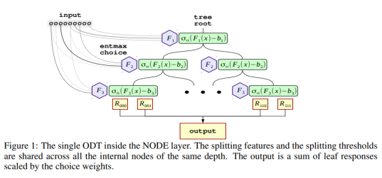
To get a feeling for how the analogy between this neural network architecture and decision tree ensembles looks, Figure 1 is reproduced here.
How should the parameters be chosen?
There is not much guidance in the manuscript; the authors suggest using hyperparameter optimization. They do mention that they optimize over the following space:
- num layers: {2, 4, 8}
- total tree count: {1024, 2048}
- tree depth: {6, 8}
- tree output dim: {2, 3}
In my code, I don’t do grid search but rather let hyperopt sample values within certain ranges. The way I thought about it (which could be wrong) is that each layer represents a tree ensemble (a single instance of CatBoost, let’s say). For each layer that you add, you may add some representation power, but you also make the model much heavier to train and potentially risk overfitting. The total tree count seems roughly analogous to the number of trees in CatBoost/xgboost/random forests, and has the same tradeoffs: with many trees, you can express more complicated functions, but the model will take much longer to train and risk overfitting. The tree depth, again, has the same type of tradeoff. As for the output dimensionality, frankly, I don’t quite understand why it is a parameter. Reading the paper, it seems it should be equal to one for regression and equal to the number of classes for classification.
How does one use NODE?
The authors have made code available on GitHub. They do not provide a command-line interface but rather suggest that users run their models in the provided Jupyter notebooks. One classification example and one regression example is provided in those notebooks.
The repo README page also strongly suggests using a GPU to train NODE models. (This is a factor in favor of CatBoost.)
I have prepared a Colaboratory notebook with some example code on how to run classification on NODE and how to optimize hyperparameters with hyperopt.
Please move to the Colaboratory notebook right now to keep following along!
Here I will just highlight some parts of the code.
General problems adapting the code
The problems I encountered when adapting the authors’ code were mainly related to data types. It’s important that the input datasets (X_train and X_val) are arrays (numpy or torch) in float32 format; not float64 or a mix of float and int. The labels need to be encoded as long (int64) for classification, and float32 for regression. (You can see this handled in the cell titled “Load, split and preprocess the data”.)
Other problems were related to memory. The models can quickly blow up the GPU memory, especially with the large batch sizes used in the authors’ example notebooks. I solved this simply by using the maximum batch size I could get away with on my laptop (and later, on Colab).
In general, though, it was not that hard to get the code to work. The documentation was a bit sparse, but sufficient.
Categorical variable handling
Unlike CatBoost, NODE does not support categorical variables, so you have to prepare those yourself into a numerical format. We do it for the Adult Census dataset in the same way the NODE authors do it, using LeaveOneOutEncoder from the category_encoders library. Here we just use a regular train/test split instead of 5-fold CV out of convenience, as it takes a long time to train NODE (especially with hyperparameter optimization).
from category_encoders import LeaveOneOutEncoder
import numpy as np
import pandas as pd
from sklearn.model_selection import train_test_split

df = pd.read_csv('https://docs.google.com/uc' +
                 '?id=10eFO2rVlsQBUffn0b7UCAp28n0mkLCy7&' +
                 'export=download')
labels = df.pop('<=50K')
X_train, X_val, y_train, y_val = train_test_split(df,
                                                  labels,
                                                  test_size=0.2)

class_to_int = {c: i for i, c in enumerate(y_train.unique())}
y_train_int = [class_to_int[v] for v in y_train]
y_val_int = [class_to_int[v] for v in y_val]

cat_features = ['workclass', 'education', 'marital-status',
                'occupation', 'relationship', 'race', 'sex',
                'native-country']

cat_encoder = LeaveOneOutEncoder()
cat_encoder.fit(X_train[cat_features], y_train_int)
X_train[cat_features] = cat_encoder.transform(X_train[cat_features])
X_val[cat_features] = cat_encoder.transform(X_val[cat_features])

# Node is going to want to have the values as float32 at some points
X_train = X_train.values.astype('float32')
X_val = X_val.values.astype('float32')
y_train = np.array(y_train_int)
y_val = np.array(y_val_int)
Now we have a fully numeric dataset.
Model definition and training loop
The rest of the code is essentially the same as in the authors’ repo (except for the hyperopt part). They created a Pytorch layer called DenseBlock, which implements the NODE architecture. A class called Trainer holds information about the experiment, and there is a straightforward training loop that keeps track of the best metrics seen so far and plots updated loss curves.
Results & conclusions
With some minimal trial and error, I was able to find a model with around 86% validation accuracy. After hyperparameter optimization with hyperopt (which was supposed to run overnight on a GPU in Colab, but in fact timed out after about 40 iterations), the best performance was 87.2%. In other runs I have achieved 87.4%. In other words, NODE did outperform CatBoost, albeit slightly, after hyperopt tuning.
However, accuracy is not everything. It is not convenient to have to do costly optimization for every dataset.
Pros of NODE vs CatBoost:
- It seems that slightly better results can be obtained (based on the NODE paper and this test; I will be sure to try many other datasets!)
Pros of CatBoost vs NODE:
- Much faster
- Less need of hyperparameter optimization
- Runs fine without GPU
- Has support for categorical variables
Which one would I use for my next projects? Probably CatBoost will still be my go-to tool, but I will keep NODE in mind and maybe try it just in case…
It’s also important to realize that performance is dataset-dependent and that the Adult Census Income dataset is not representative of all scenarios. Perhaps more importantly, the preprocessing of categorical features is likely rather important in NODE. I’ll return to the subject of preprocessing in a future post!

