Modelling tabular data with Google’s TabNet

Released in 2019, Google Research’s TabNet is claimed in a preprint manuscript to outperform existing methods on tabular data. How does it work and how can one try it?

Tabular data probably make up the majority of business data today. Think of things like retail transactions, click stream data, temperature and pressure sensors in factories, KYC information… the variety is endless.

In another post, I introduced CatBoost, one of my favorite methods for building prediction models on tabular data, and its neural network counterpart, NODE. But around the same time as the NODE manuscript came out, Google Research released a manuscript taking a totally different approach to tabular data modelling with neural networks. Whereas NODE mimics decision tree ensembles, Google’s proposed TabNet tries to build a new kind of architecture suitable for tabular data.

The paper describing the method is called TabNet: Attentive Interpretable Tabular Learning, which nicely summarizes what the authors are trying to do. The “Net” part tells us that it is a type of neural network, the “Attentive” part implies it is using an attention mechanism, it aims to be interpretable, and it is used for machine learning on tabular data.

How does it work?

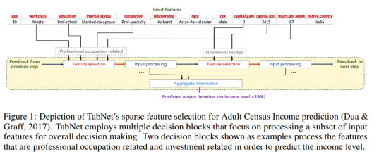
TabNet uses a kind of soft feature selection to focus on just the features that are important for the example at hand. This is accomplished through a sequential multi-step decision mechanism. That is, the input information is processed top-down in several steps. As the manuscript puts it, “The idea of top-down attention in sequential form is inspired from its applications in processing visual and language data such as for visual question answering (Hudson & Manning, 2018) or in reinforcement learning (Mott et al., 2019) while searching for a small subset of relevant information in high dimensional input.”

The building blocks for performing this sequential attention are called transformer blocks even though they are a bit different from the transformers used in popular NLP models such as BERT. The soft feature selection is accomplished by using the sparsemax function.

The first figure from the paper, reproduced below, sketches how information is aggregated to form a prediction.

One nice property of TabNet is that it does not require feature preprocessing (in contrast to e.g. NODE). Another one is that it has interpretability built in “for free” in that the most relevant features are selected for each example. This means that you don’t have to apply an external explanation module such as shap or LIME.

It is not so easy to wrap one’s head around what is happening inside this architecture when reading the paper, but luckily there is published code which clarifies things a bit and shows that it is not as complicated as you might think.

How can I use it?

 

The original code and modifications

As already mentioned, the code is available, and the authors show how to use it together with the forest covertype dataset. To facilitate this, they have provided three dataset-specific files: one file that downloads and prepares the data (download_prepare_covertype.py), another one that defines the appropriate Tensorflow Feature Columns and a CSV reader input function (data_helper_covertype.py), and the file that contains the training loop (experiment_covertype.py).

The repo README states:

To modify the experiment to other tabular datasets:

– Substitute the train.csv, val.csv, and test.csv files under “data/” directory,

– Modify the data_helper function with the numerical and categorical features of the new dataset,

– Reoptimize the TabNet hyperparameters for the new dataset.

After having gone through this process a couple of times with other datasets, I decided to write my own wrapper code to streamline the process. This code, which I must stress is a totally unofficial fork, is on GitHub.

In terms of the README points above:

• Rather than making new train.csv, val.csv and test.csv files for each dataset, I preferred to read the entire dataset and do the splitting in-memory (as long as it is feasible, of course), so I wrote a new input function for Pandas in my code.
• It can take a bit of work to modify the data_helper.py file, at least initially when you aren’t quite sure what it does and how the feature columns should be defined (this was certainly the case with me). There are also many parameters which need to be changed but which are in the main training loop file rather than the data helper file. In view of this, I also tried to generalize and streamline this process in my code.
• I added some quick-and-dirty code for doing hyperparameter optimization, but so far only for classification.
• It is also worth mentioning that the example code from the authors only shows how to do classification, not regression, so that extra code also has to be written by the user. I have added regression functionality with a simple mean squared error loss.

Using the command-line interface

Execute a command like:

python train_tabnet.py \
  --csv-path data/adult.csv \
  --target-name "<=50K" \
  --categorical-features workclass,education,marital.status,\
occupation,relationship,race,sex,native.country\
  --feature_dim 16 \
  --output_dim 16 \
  --batch-size 4096 \
  --virtual-batch-size 128 \
  --batch-momentum 0.98 \
  --gamma 1.5 \
  --n_steps 5 \
  --decay-every 2500 \
  --lambda-sparsity 0.0001 \
  --max-steps 7700

The mandatory parameters are — -csv-path(pointing to the location of the CSV file),--target-name(the name of the column with the prediction target) and--categorical-featues (a comma-separated list of the features that should be treated as categorical). The rest of the input parameters are hyperparameters that need to be optimized for each specific problem. The values shown above, though, are taken directly from the TabNet manuscript, so they have already been optimized for the Adult Census dataset by the authors.

By default, the training process will write information to the tflog subfolder of the location where you execute the script. You can point tensorboard at this folder to look at training and validation stats:

tensorboard --logdir tflog

and point your web browser to localhost:6006.

If you don’t have a GPU…

… you could try this Colaboratory notebook. Note that if you want to look at the Tensorboard logs, your best bet is probably to create a Google Storage bucket and have the script write the logs there. This is accomplished by using the tb-log-locationparameter. E.g. if your bucket’s name were camembert-skyscrape, you could add--tb-log-location gs://camembert-skyscraperto the invocation of the script. (Note, though, that you have to set the permissions for the storage bucket correctly. This can be a bit of a hassle.)

Then you can point tensorboard, from your own local computer, to that bucket:

tensorboard --logdir gs://camembert-skyscraper

Hyperparameter optimization

There is also a quick-and-dirty script for doing hyperparameter optimization in the repo (opt_tabnet.py). Again, an example is shown in the Colaboratory notebook. The script only works for classification so far, and it is worth noting that some training parameters are still hard-coded although they shouldn’t really be (for example, the patience parameter for early stopping [how many steps do you continue while the best validation accuracy does not improve].)

The parameters that are varied in the optimization script are N_steps, feature_dim, batch-momentum, gamma, lambda-sparsity. (output_dim is set to be equal to feature_dim, as suggested in the optimization tips just below.)

The paper has the following tips on hyperparameter optimization:

Most datasets yield the best results for N_steps ∈ [3, 10]. Typically, larger datasets and more complex tasks require a larger N_steps. A very high value of N_steps may suffer from overfitting and yield poor generalization.

Adjustment of the values of Nd [feature_dim] and Na [output_dim] is the most efficient way of obtaining a trade-off between performance and complexity. Nd = Na is a reasonable choice for most datasets. A very high value of Nd and Na may suffer from overfitting and yield poor generalization.

An optimal choice of γ can have a major role on the overall performance. Typically a larger N_steps value favors for a larger γ.

A large batch size is beneficial for performance — if the memory constraints permit, as large as 1–10 % of the total training dataset size is suggested. The virtual batch size is typically much smaller than the batch size.

Initially large learning rate is important, which should be gradually decayed until convergence.

Results

I’ve tried TabNet via this command line interface for several datasets, including the Adult Census dataset that I used in the post about NODE and CatBoost for reasons that can be found in that post. Conveniently, this dataset had also been used in the TabNet manuscript, and the authors present the best parameter settings they found there. With repeated runs using those setting, I noticed that the best validation error (and test error) tends to be at around 86%, similar to CatBoost without hyperparameter tuning. The authors report a test set performance of 85.7% in the manuscript. When I did hyperparameter optimization with hyperopt, I unsurprisingly reached a similar performance around 86%, albeit with a different parameter setting.

For other datasets such as the Poker Hand dataset, TabNet is claimed to beat other methods by a considerable margin. I have not yet devoted much time to that, but everyone is of course invited to try TabNet with hyperparameter optimization on various datasets for themselves!

Conclusions

TabNet is an interesting architecture that seems promising for tabular data analysis. It operates directly on raw data and uses a sequential attention mechanism to perform explicit feature selection for each example. This property also gives it a sort of built-in interpretability.

I have tried to make TabNet slightly easier to work with by writing some wrapper code around it. The next step is to compare it to other methods across a wide range of datasets.

Please try it on your own datasets and/or send pull requests and help me improve the interface if you are interested!

 

Modelling tabular data with CatBoost and NODE

CatBoost from Yandex, a Russian online search company, is fast and easy to use, but recently researchers from the same company released a new neural network based package, NODE, that they claim outperforms CatBoost and all other gradient boosting methods. Can this be true? Let’s find out how to use both CatBoost and NODE!

Who is this blog post for?

Although I wrote this blog post for anyone who is interested in machine learning and in particular tabular data, it is helpful if you are familiar with Python and the scikit-learn library if you want to follow along with the code. If you aren’t, hopefully you will find the theoretical and conceptual parts interesting anyway!

CatBoost introduction

CatBoost is my go-to package for modelling tabular data. It is an implementation of gradient boosted decision trees with a few tweaks that make it slightly different from e.g. xgboost or LightGBM. It works for both classification and regression problems.

Some nice things about CatBoost:

• It handles categorical features (get it?) out of the box, so you don’t need to worry about how to encode them.
• It typically requires very little parameter tuning.
• It avoids certain subtle types of data leakage that other methods may suffer from. 
• It is fast, and can be run on GPU if you want it to go even faster.

These factors make CatBoost, for me, a no-brainer as the first thing to reach for when I need to analyze a new tabular dataset.

Technical details of CatBoost

Skip this section if you just want to use CatBoost!

On a more technical level, there are some interesting things about how CatBoost is implemented. I highly recommend the paper Catboost: unbiased boosting with categorical features if you are interested in the details. I just want to highlight two things.

1. In the paper, the authors show that standard gradient boosting algorithms are affected by subtle types of data leakage which result from the way that the models are iteratively fitted. In a similar manner, the most effective ways to encode categorical features numerically (like target encoding) are prone to data leakage and overfitting. To avoid this leakage, CatBoost introduces an artificial timeline according to which the training examples arrive, so that only “previously seen” examples can be used when calculating statistics.
2. CatBoost actually doesn’t use regular decision trees, but oblivious decision trees. These are trees where, at each level of the tree, the same feature and the same splitting criterion is used everywhere! This sounds weird, but has some nice properties. Let’s look at what is meant by this.

Regular decision tree. Any feature or split point can be present at each level.

Oblivious decision tree. Each level has the same splits.

Left: Regular decision tree. Any feature or split point can be present at each level. Right: Oblivious decision tree. Each level has the same splits.

In a normal decision tree, feature to split on and the cutoff value both depend on what path you have taken so far in the tree. This makes sense, because we can use the information we already have to decide the most informative next question (like in the “20 questions” game). With oblivious decision trees, the history doesn’t matter; we pose the same question no matter what. The trees are called “oblivious” because they keep “forgetting” what has happened before. 

Why is this useful? One nice property of oblivious decision trees is that an example can be classified or scored really quickly – it is always the same N binary questions that are posed (where N is the depth of the tree). This can easily be done in parallel for many examples. That is one reason why CatBoost is fast. Another thing to keep in mind is that we are dealing with a tree ensemble here. As a stand-alone algorithm, the oblivious decision tree might not work so well, but the idea of tree ensembles is that a coalition of weak learners often works well because errors and biases are “washed out”. Normally, the weak learner is a standard decision tree, and here it is something even weaker, namely the oblivious decision tree. The CatBoost authors argue that this particular weak base learner works well for generalization.

Installing CatBoost

Although installing CatBoost should be a simple matter of typing

pip install catboost

I’ve sometimes encountered problems with that when on a Mac. On Linux systems such as the Ubuntu system I am typing on now, or on Google Colaboratory, it should “just work”. If you keep having problems installing it, consider using a Docker image, e.g.

docker pull yandex/tutorial-catboost-clickhouse
docker run -it yandex/tutorial-catboost-clickhouse

Using CatBoost on a dataset

Link to Colab notebook with code

Let’s have a look at how to use CatBoost on a tabular dataset. We start by downloading a lightly preprocessed version of the Adult/Census Income  dataset which is, in the following, assumed to be located in datasets/adult.csv. I chose this dataset because it has a mix of categorical and numerical features, a nice manageable size in the tens of thousands of examples and not too many features. It is often used to exemplify algorithms, for instance in Google’s What-If Tool and many other places.  

The adult census dataset has the columns ‘age’, ‘workclass’, ‘education’, ‘education-num’, ‘marital-status’, ‘occupation’, ‘relationship’, ‘race’, ‘sex’, ‘capital-gain’, ‘capital-loss’, ‘hours-per-week’, ‘native-country’, and ‘<=50K‘. The task is to predict the value of the last column, ‘<=50K’, which indicates if the person in question earns 50,000 USD or less per year (the dataset is from 1994). We regard the following features as categorical rather than numerical: ‘workclass’, ‘education’, ‘marital-status’, ‘occupation’, ‘relationship’, ‘race’, ‘sex’, ‘native-country’.

The code is pretty similar to scikit-learn except for the Pool datatype that CatBoost uses to bundle feature and target values for a dataset while keeping them conceptually separate. (I have to admit I don’t really know why Pool is there – I just use it, and it seems to work fine.)

The code is available on Colab, but I will copy it here for reference. CatBoost needs to know which features are categorical and will then handle them automatically. In this code snippet, I also use 5-fold (stratified) cross-validation to estimate the prediction accuracy.

from catboost import CatBoostClassifier, Pool
from hyperopt import fmin, hp, tpe
import pandas as pd
from sklearn.model_selection import StratifiedKFold

df = pd.read_csv("https://docs.google.com/uc?" + 
                 "id=10eFO2rVlsQBUffn0b7UCAp28n0mkLCy7&" + 
                 "export=download")
labels = df.pop('<=50K')

categorical_names = ['workclass', 'education', 'marital-status',
                     'occupation', 'relationship', 'race',
                     'sex', 'native-country']  
categoricals = [df.columns.get_loc(i) for i in categorical_names]

nfolds = 5
skf = StratifiedKFold(n_splits=nfolds, shuffle=True)
acc = []

for train_index, test_index in skf.split(df, labels):
  X_train, X_test = df.iloc[train_index].copy(), \
                    df.iloc[test_index].copy()
  y_train, y_test = labels.iloc[train_index], \
                    labels.iloc[test_index]
  train_pool = Pool(X_train, y_train, cat_features = categoricals)
  test_pool = Pool(X_test, y_test, cat_features = categoricals)
  model = CatBoostClassifier(iterations=100,
                             depth=8,
                             learning_rate=1,
                             loss_function='MultiClass') 
  model.fit(train_pool)
  predictions = model.predict(test_pool)
  accuracy = sum(predictions.squeeze() == y_test) / len(predictions)
  acc.append(accuracy)

mean_acc = sum(acc) / nfolds
print(f'Mean accuracy based on {nfolds} folds: {mean_acc:.3f}')
print(acc)

What we tend to get from running this (CatBoost without hyperparameter optimization) is a mean accuracy between 85% and 86%. In my last run, I got about 85.7%.

If we want to try to optimize the hyperparameters, we can use hyperopt (if you don’t have it, install it with pip install hyperopt). In order to use it, you need to define a function that hyperopt tries to minimize. We will just try to optimize the accuracy here. Perhaps it would be better to optimize e.g. log loss, but that is left as an exercise to the reader 😉 

The main parameters to optimize are probably the number of iterations, the learning rate, and the tree depth. There are also many other parameters related to over-fitting, for instance early stopping rounds and so on. Feel free to explore on your own!

# Optimize between 10 and 1000 iterations and depth between 2 and 12

search_space = {'iterations': hp.quniform('iterations', 10, 1000, 10),
                'depth': hp.quniform('depth', 2, 12, 1),
                'lr': hp.uniform('lr', 0.01, 1)
               }

def opt_fn(search_space):

  nfolds = 5
  skf = StratifiedKFold(n_splits=nfolds, shuffle=True)
  acc = []

  for train_index, test_index in skf.split(df, labels):
    X_train, X_test = df.iloc[train_index].copy(), \
                      df.iloc[test_index].copy()
    y_train, y_test = labels.iloc[train_index], \
                      labels.iloc[test_index]
    train_pool = Pool(X_train, y_train, cat_features = categoricals)
    test_pool = Pool(X_test, y_test, cat_features = categoricals)

    model = CatBoostClassifier(iterations=search_space['iterations'],
                             depth=search_space['depth'],
                             learning_rate=search_space['lr'],
                             loss_function='MultiClass',
                             od_type='Iter')

    model.fit(train_pool, logging_level='Silent')
    predictions = model.predict(test_pool)
    accuracy = sum(predictions.squeeze() == y_test) / len(predictions)
    acc.append(accuracy)

  mean_acc = sum(acc) / nfolds
  return -1*mean_acc

best = fmin(fn=opt_fn, 
            space=search_space, 
            algo=tpe.suggest, 
            max_evals=100)

When I last ran this code, it took over 5 hours but resulted in a mean accuracy of 87.3%, which is on par with the best results I got when trying the Auger.ai AutoML platform.

Sanity check: logistic regression

At this point we should ask ourselves if these fancy new-fangled methods are really needed. How would a good old logistic regression perform out of the box and after hyperparameter optimization?

I’ll omit reproducing the code here for brevity’s sake, but it is available in the same Colab notebook as before. One detail with the logistic regression implementation is that it doesn’t handle categorical variables out of the box like CatBoost does, so I decided to code them using target encoding, specifically leave-one-out target encoding, which is the approach taken in NODE and a fairly close though not identical analogue of what happens in CatBoost.

Long story short, untuned logistic regression with this type of encoding yields around 80% accuracy, and around 81% (80.7% in my latest run) after hyperparameter tuning. Here, an interestin alternative is to try automated preprocessing libraries such as vtreat and Automunge, but I will save those for an upcoming blog post!

Taking stock

What do we have so far, before trying NODE?

• Logistic regression, untuned: 80.0%
• Logistic regression, tuned: 80.7%
• CatBoost, untuned: 85.7%
• CatBoost, tuned: 87.2%

 

NODE: Neural Oblivious Decision Ensembles

A recent manuscript from Yandex researchers describes an interesting neural network version of CatBoost, or at least a neural network take on oblivious decision tree ensembles (see the technical section above if you want to remind yourself what “oblivious” means here.) This architecture, called NODE, can be used for either classification or regression.

One of the claims from the abstract reads: “With an extensive experimental comparison to the leading GBDT packages on a large number of tabular datasets, we demonstrate the advantage of the proposed NODE architecture, which outperforms the competitors on most of the tasks.” This naturally piqued my interest. Could this tool be better than CatBoost?

How does NODE work?

You should go to the paper for the full story, but some relevant details are:

• The entmax activation function is used as a soft version of a split in a regular decision tree. As the paper puts it, “The entmax is capable to produce sparse probability distributions, where the majority of probabilities are exactly equal to 0. In this work, we argue that entmax is also an appropriate inductive bias in our model, which allows differentiable split decision construction in the internal tree nodes. Intuitively, entmax can learn splitting decisions based on a small subset of data features (up to one, as in classical decision trees), avoiding undesired influence from others.” The entmax functions allows a neural network to mimic a decision tree-type system while keeping the model differentiable (weights can be updated based on the gradients).
• The authors present a new type of layer, a “node layer”, which you can use in a neural network (their implementation is in PyTorch). A node layer represents a tree ensemble.
• Several node layers can be stacked, yielding a hierarchical model where the input is fed through one tree ensemble at a time. Successive concatenation of input representations can be used to give a model which is reminiscent of the popular DenseNet model for image processing, just specialized in tabular data.
• The parameters of a NODE model are:
  • Learning rate (always 0.001 in the paper)
  • The number of node layers (k)
  • The number of trees in each layer (m)
  • The depth of the trees in each layer (d)

 

How is NODE related to tree ensembles?

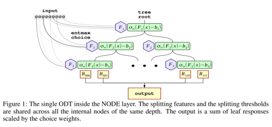
To get a feeling for how the analogy between this neural network architecture and decision tree ensembles looks, Figure 1 is reproduced here.

How should the parameters be chosen?

There is not much guidance in the manuscript; the authors suggest using hyperparameter optimization. They do mention that they optimize over the following space:

• num layers: {2, 4, 8} 
• total tree count: {1024, 2048} 
• tree depth: {6, 8} 
• tree output dim: {2, 3}

In my code, I don’t do grid search but rather let hyperopt sample values within certain ranges. The way I thought about it (which could be wrong) is that each layer represents a tree ensemble (a single instance of CatBoost, let’s say). For each layer that you add, you may add some representation power, but you also make the model much heavier to train and potentially risk overfitting. The total tree count seems roughly analogous to the number of trees in CatBoost/xgboost/random forests, and has the same tradeoffs: with many trees, you can express more complicated functions, but the model will take much longer to train and risk overfitting. The tree depth, again, has the same type of tradeoff. As for the output dimensionality, frankly, I don’t quite understand why it is a parameter. Reading the paper, it seems it should be equal to one for regression and equal to the number of classes for classification.

How does one use NODE?

The authors have made code available on GitHub. They do not provide a command-line interface but rather suggest that users run their models in the provided Jupyter notebooks. One classification example and one regression example is provided in those notebooks.

The repo README page also strongly suggests using a GPU to train NODE models. (This is a factor in favor of CatBoost.) 

I have prepared a Colaboratory notebook with some example code on how to run classification on NODE and how to optimize hyperparameters with hyperopt. 

Please move to the Colaboratory notebook right now to keep following along! 

Here I will just highlight some parts of the code.

General problems adapting the code

The problems I encountered when adapting the authors’ code were mainly related to data types. It’s important that the input datasets (X_train and X_val) are arrays (numpy or torch) in float32 format; not float64 or a mix of float and int. The labels need to be encoded as long (int64) for classification, and float32 for regression. (You can see this handled in the cell titled “Load, split and preprocess the data”.)

Other problems were related to memory. The models can quickly blow up the GPU memory, especially with the large batch sizes used in the authors’ example notebooks. I solved this simply by using the maximum batch size I could get away with on my laptop (and later, on Colab).

In general, though, it was not that hard to get the code to work. The documentation was a bit sparse, but sufficient.

 

Categorical variable handling

Unlike CatBoost, NODE does not support categorical variables, so you have to prepare those yourself into a numerical format. We do it for the Adult Census dataset in the same way the NODE authors do it, using LeaveOneOutEncoder from the category_encoders library. Here we just use a regular train/test split instead of 5-fold CV out of convenience, as it takes a long time to train NODE (especially with hyperparameter optimization).

from category_encoders import LeaveOneOutEncoder
import numpy as np
import pandas as pd
from sklearn.model_selection import train_test_split

df = pd.read_csv('https://docs.google.com/uc' + 
                 '?id=10eFO2rVlsQBUffn0b7UCAp28n0mkLCy7&' + 
                 'export=download')
labels = df.pop('<=50K')
X_train, X_val, y_train, y_val = train_test_split(df,
                                                  labels,
                                                  test_size=0.2)

class_to_int = {c: i for i, c in enumerate(y_train.unique())}                                                                                                               
y_train_int = [class_to_int[v] for v in y_train]                                                                                                                            
y_val_int = [class_to_int[v] for v in y_val] 

cat_features = ['workclass', 'education', 'marital-status',
                'occupation', 'relationship', 'race', 'sex',
                'native-country']
  
cat_encoder = LeaveOneOutEncoder()
cat_encoder.fit(X_train[cat_features], y_train_int)
X_train[cat_features] = cat_encoder.transform(X_train[cat_features])
X_val[cat_features] = cat_encoder.transform(X_val[cat_features])

# Node is going to want to have the values as float32 at some points
X_train = X_train.values.astype('float32')
X_val = X_val.values.astype('float32')
y_train = np.array(y_train_int)
y_val = np.array(y_val_int)

Now we have a fully numeric dataset. 

Model definition and training loop

The rest of the code is essentially the same as in the authors’ repo (except for the hyperopt part). They created a Pytorch layer called DenseBlock, which implements the NODE architecture. A class called Trainer holds information about the experiment, and there is a straightforward training loop that keeps track of the best metrics seen so far and plots updated loss curves.

Results & conclusions

With some minimal trial and error, I was able to find a model with around 86% validation accuracy. After hyperparameter optimization with hyperopt (which was supposed to run overnight on a GPU in Colab, but in fact timed out after about 40 iterations), the best performance was 87.2%. In other runs I have achieved 87.4%. In other words, NODE did outperform CatBoost, albeit slightly, after hyperopt tuning.

However, accuracy is not everything. It is not convenient to have to do costly optimization for every dataset. 

Pros of NODE vs CatBoost:

• It seems that slightly better results can be obtained (based on the NODE paper and this test; I will be sure to try many other datasets!)

Pros of CatBoost vs NODE:

• Much faster
• Less need of hyperparameter optimization
• Runs fine without GPU
• Has support for categorical variables

Which one would I use for my next projects? Probably CatBoost will still be my go-to tool, but I will keep NODE in mind and maybe try it just in case…

It’s also important to realize that performance is dataset-dependent and that the Adult Census Income dataset is not representative of all scenarios. Perhaps more importantly, the preprocessing of categorical features is likely rather important in NODE. I’ll return to the subject of preprocessing in a future post!

 

Tutorial: Exploring TCGA breast cancer proteomics data

Data used in this publication were generated by the Clinical Proteomic Tumor Analysis Consortium (NCI/NIH).

The Cancer Genome Atlas (TCGA) has become a focal point for a lot of genomics and bioinformatics research. DNA and RNA level data on different tumor types are now used in countless papers to test computational methods and to learn more about hallmarks of different types of cancer.

Perhaps, though, there aren’t as many people who are using the quantitative proteomics data hosted by Clinical Proteomic Tumor Analysis Consortium (CPTAC). There are mass spectrometry based expression measurements for many different types of tumor available at their Data Portal.

As I have been comparing some (currently in-house, to be published eventually) cancer proteomics data sets against TCGA proteomics data, I thought I would share some code, tricks and tips for those readers who want to start analyzing TCGA data (whether proteomics, transcriptomics or other kinds) but don’t quite know where to start.

To this end, I have put a tutorial Jupyter notebook at Github: TCGA protein tutorial

The tutorial is written in R, mainly because I like the TCGA2STAT and Boruta packages (but I just learned there is a Boruta implementation in Python as well.) If you think it would be useful to have a similar tutorial in Python, I will consider writing one.

The tutorial consists, roughly, of these steps:

• Getting a usable set of breast cancer proteomics data
  This consists of downloading the data, selecting the subset that we want to focus on, removing features with undefined values, etc..
• Doing feature selection to find proteins predictive of breast cancer subtype.
  Here, the Boruta feature selection package is used to identify a compact set of proteins that can predict the so-called PAM50 subtype of each tumor sample. (The PAM50 subtype is based on mRNA expression levels.)
• Comparing RNA-seq data and proteomics data on the same samples.
  Here, we use the TCGA2STAT package to obtain TCGA RNA-seq data and find the set of common gene names and common samples between our protein and mRNA-seq data in order to look at protein-mRNA correlations.

Please visit the notebook if you are interested!

Some of the take-aways from the tutorial may be:

• A bit of messing about with metadata, sample names etc. is usually necessary to get the data in the proper format, especially if you are combining different kinds of data (such as RNA-seq and proteomics here). I guess you’ve heard them say that 80% of data science is data preparation!…
• There are now quantitative proteomics data available for many types of TCGA tumor samples.
• TCGA2STAT is a nice package for importing certain kinds of TCGA data into an R session.
• Boruta is an interesting alternative for feature selection in a classification context.

This post was prepared with permission from CPTAC.

P.S. I may add some more material on a couple of ways to do multivariate data integration on TCGA data sets later, or make that a separate blog post. Tell me if you are interested.

Notes on genomics APIs #3: SolveBio

This is the third in a short series of posts with notes on different genomics APIs. The first post, which was about the One Codex API, can be found here, and the second one, about Google Genomics, can be found here.

SolveBio “delivers the critical reference data used by hospitals and companies to run genomic applications”, according to their web page. They focus on clinical genomics and on helping developers who need to access various data sources in a programmatic way. Their curated data library provides access to (as of February 2015) “over 300 datasets for genomics, proteomics, literature annotation, variant-disease relationships, and more.) Some examples of those datasets are the ClinVar disease gene database from NIH, the Somatic Mutations dataset from The Cancer Genome Atlas, and the COSMIC catalogue of somatic mutations in cancer.

SolveBio offers a RESTful API with Python and Ruby clients already available and an R client under development. The Getting Started Guide really tells you most of what you need to know to use it, but let’s try it out here on this blog anyway!

You should, of course, start by signing up for a free account. After that, it’s time to get the client. I will use the Python one in this post. It can be installed by giving this command:

curl -skL install.solvebio.com/python | bash

You can also install it with pip.

Now you will need to login. This will prompt you for your email and password that you registered when signing up.

solvebio login

At this point you can view a useful tutorial by giving solvebio tutorial. The tutorial explains the concept of depositories, which are versioned containers for data sets. For instance (as explained in the docs), there is a ClinVar depository which (as of version 3.1.0) has three datasets: ClinVar, Variants, and Submissions. Each dataset within a depository is designed for a specific use-case. For example, the Variants dataset contains data on genomic variants, and supports multiple genome builds.

Now start the interactive SolveBio shell. This shell (in case you followed the instructions above) is based on iPython.

solvebio


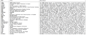
The command Depository.all() will show the available depositories. Currently, the list looks like this (you’ll want to click the image to blow it up a bit):

In a similar way, you can view all the data sets with Dataset.all(). Type Dataset.all(latest=True) to view only the latest additions.

To work with a data set, you need to ‘retrieve’ it with a command like:

ds = Dataset.retrieve('ClinVar/3.1.0-2015-01-13/Variants')

It is perfectly possible to leave out the version of the data set: ds = Dataset.retrieve('ClinVar/Variants') but that is bad practice from a reproducibility viewpoint and is not recommended, especially in production code.

Now we can check which fields are available in the ds object representing the data set we selected.

ds.fields()

There are fields for things like alternate alleles for the variant in question, sources of clinical information on the variant, the name of any gene(s) overlapping the variant, and the genomic coordinates for the variant.

You can create a Python iterator for looping through all the records (variants) using ds.query(). To view the first variant, type ds.query()[0]. This will give you an idea of how each record (variant) is described in this particular data set. In practice, you will almost always want to filter your query according to some specified criteria. So for example, to look for known pathogenic variants in the titin (TTN) gene, you could filter as follows:

ttn_vars = ds.query().filter(clinical_significance='Pathogenic', gene_symbol_hgnc='TTN')

This will give you an iterator with a bunch of records (currently 18) that you can examine in more detail.

If you want to search for variants in some specified genomic region that you have identified as interesting, you can do that too, but it is only possible for some data sets. In this case it turns out that we can do it with this version of the ClinVar variant data set, because it is considered a “genomic” data set, which we can see because the command ds.is_genomicreturns True. (Some of the older versions return False here.)

ds.query(genome_build='GRCh37').range('chr3', 22500000, 23000000)

Note that you can specify a genome build in the query, which is very convenient.

Moving on to a different depository and data set, we can search for diabetes-related variants as defined via genome wide association studies with something like the following:

ds = Dataset.retrieve('GWAS/1.0.0-2015-01-13/GWAS')
ds.fields() # Check out which fields are available
ds.query().filter(phenotype='diabetes') # Also works with "Diabetes"
ds.query().filter(journal='science',phenotype='diabetes') # Only look for diabetes GWAS published in Science


Also, giving a command likeDataset.retrieve('GWAS/1.0.0-2015-01-13/GWAS').help() will open up a web page describing the dataset in your browser.

Notes on genomics APIs #2: Google Genomics API

This is the second in a series of about three posts with notes on different genomics APIs. The first post, which was about the One Codex API, can be found here.

As you may have heard, Google has started building an ambitious infrastructure for storing and querying genomic data, so I was eager to start exploring it. However, as there were a number of tools available, I initially had some trouble wrapping my head around what I was supposed to do. I hope these notes, where I mainly use the API for R, can provide some help.

Some useful bookmarks:

Google Developers Console – for creating and managing Google Genomics and BigQuery projects.

Google Genomics GitHub repo

Google Cloud Platform Google Genomics page (not sure what to call this page really)

Getting started

You should start by going to the Developer Console and creating a project. You will need to give it a name, and in addition it will be given a unique ID which you can use later in API calls. When the project has been created, click “Enable an API” on the Dashboard page, and click the button where it says “OFF” next to Genomics API (you may need to scroll down to find it).

Now you need to create a client_secret.json file that you will use for some API calls. Click the Credentials link in the left side panel and then click “Create new client ID”. Select “Installed application” and fill in the “Consent screen” form. All you really need to do is select an email address and type a “product name”, like “BlogTutorial” like I did for this particular example. Select “Installed application” again if you are prompted to select an application type. Now it should display some information under the heading “Client ID for native application”. Click the “Download JSON” button and rename the file to client_secret.json. (I got these instructions from here.)

Using the Java API client for exploring the data sets

One of the first questions I had was how to find out which datasets are actually available for querying. Although it is perfectly possible to click around in the Developer Console, I think the most straightforward way currently is to use the Java API client. I installed it from the Google Genomics GitHub repo by cloning:
git clone git@github.com:googlegenomics/api-client-java.git
The GitHub repo page contains installation instructions, but I will repeat them here. You need to compile it using Maven:

cd api-client-java
mvn package

If everything goes well, you should now be able to use the Java API client to look for datasets. It is convenient (but not necessary) to put the client_secret.json file into the same directory as the Java API client. Let’s check which data sets are available (this will only work for projects where billing has been enabled; you can sign up for a free trial in which case you will not be surprise-billed):

java -jar genomics-tools-client-java-v1beta2.jar listdatasets --project_number 761052378059 --client_secrets_filename client_secret.json


(If your client_secret.json file is in another directory, you need to give the full path to the file, of course.) The project number is shown on your project page in the Developer Console. Now, the client will open a browser window where you need to authenticate. You will only need to do this the first time. Finally, the results are displayed. They currently look like this:

Platinum Genomes (ID: 3049512673186936334)
1000 Genomes - Phase 3 (ID: 4252737135923902652)
1000 Genomes (ID: 10473108253681171589)


So there are three data sets. Now let’s check which reference genomes are available:

java -jar genomics-tools-client-java-v1beta2.jar searchreferencesets --client_secrets_filename ../client_secret.json --fields 'referenceSets(id,assemblyId)'


The output is currently:

{"assemblyId":"GRCh37lite","id":"EJjur6DxjIa6KQ"}
{"assemblyId":"GRCh38","id":"EMud_c37lKPXTQ"}
{"assemblyId":"hs37d5","id":"EOSt9JOVhp3jkwE"}
{"assemblyId":"GRCh37","id":"EOSsjdnTicvzwAE"}
{"assemblyId":"hg19","id":"EMWV_ZfLxrDY-wE"}


To find out the names of the chromosomes/contigs in one of the reference genomes: (by default this will only return the ten first hits, so I specify –count 50)

java -jar genomics-tools-client-java-v1beta2.jar searchreferences --client_secrets_filename client_secret.json  --fields 'references(id,name)' --reference_set_id EMWV_ZfLxrDY-wE --count 50


Now we can try to extract a snippet of sequence from one of the chromosomes. Chromosome 9 in hg19 had the ID EIeX4KDCl634Jw, so the query becomes, if we want to extract some sequence from 13 Mbases into the chromosome:

java -jar genomics-tools-client-java-v1beta2.jar getreferencebases  --client_secrets_filename client_secret.json --reference_id ENywqdu-wbqQBA --start 13000000 --end 13000070


This returns the sequence AGGGACAGGAATTGAGATTTAGGAAGCCATCAGGACTTGGGTTTTTGTCATCCCACTCTATTTCTCTCTG.

Another thing you might want to do is to check which “read groups” that are available in one of the data sets. For instance, for the Platinum Genomes data set we get:

java -jar genomics-tools-client-java-v1beta2.jar searchreadgroupsets --dataset_id 3049512673186936334  --client_secrets_filename client_secret.json


which outputs a bunch of JSON records that show the corresponding sample name, BAM file, internal IDs, software and version used for alignment to the reference genome, etc.

Using BigQuery to search Google Genomics data sets

Now let’s see how we can call the API from R. The three data sets mentioned above can be queried using Google’s BigQuery interface, which allows SQL-like queries to be run on very large data sets. Start R and install and load some packages:

install.packages("devtools") # unless you already have it!
library("devtools")
devtools::install_github("hadley/assertthat")
devtools::install_github("hadley/bigrquery")
library("bigrquery")

Now we can access BigQuery through R. Try one of the non-genomics data sets just to get warmed up.

project <- '(YOUR_PROJECT_ID)' # the ID of the project from the Developer Console
sql <- 'SELECT title,contributor_username,comment FROM[publicdata:samples.wikipedia] WHERE title contains "beer" LIMIT 100;'
data <- query_exec(sql, project)


Now the data object should contain a list of Wikipedia articles about beer. If that worked, move on to some genomic queries. In this case, I decided I wanted to look at the SNP for the photic sneeze reflex (the reflex that makes people such as myself sneeze when they go out on a sunny day) that 23andme discovered via their user base. That genetic variant has the ID and is located on chromosome 2, base 146125523 in the hg19 reference genome. It seems that 23andme uses a 1-based coordinate system (the first nucleotide has the index 1) while Google Genomics uses a 0-based system, so we should look for base position 146125522 instead. We query the Platinum Genomes variant table: (you can find the available tables at the BigQuery Browser Tool Page)

sql <- 'SELECT reference_bases,alternate_bases FROM[genomics-public-data:platinum_genomes.variants] WHERE reference_name="chr2" AND start=146125522 GROUP BY reference_bases,alternate_bases;'
query_exec(sql, project)

This shows the following output:

reference_bases alternate_bases
1 C T

This seems to match the description provided by 23andme; the reference allele is C and the most common alternate allele is T. People with CC have slightly higher odds of sneezing in the sun, TT people have slightly lower odds, and people with CT have average odds.

If we query for the variant frequencies (VF) in the 13 Platinum genomes, we get the following results (the fraction represents, as I interpret it, the fraction of sequencing reads that has the “alternate allele”, in this case T):

sql <- 'SELECT call.call_set_name,call.VF FROM[genomics-public-data:platinum_genomes.variants] WHERE reference_name="chr2" AND start=146125522;'
query_exec(sql, project)

The output is as follows:

call_call_set_name call_VF
1 NA12882 0.500
2 NA12877 0.485
3 NA12889 0.356
4 NA12885 1.000
5 NA12883 0.582
6 NA12879 0.434
7 NA12891 1.000
8 NA12888 0.475
9 NA12886 0.434
10 NA12884 0.459
11 NA12893 0.588
12 NA12878 0.444
13 NA12892 0.533

So most people here seem to have a mix of C and T, with two individuals (NA12891 and NA12885) having all T:s, in other words they appear to be homozygous for the T allele, if I am interpreting this correctly.

Using the R API client

Now let’s try to use the R API client. In R, install the client from GitHub, and also ggbio and ggplot2 if you don’t have them already:

source("http://bioconductor.org/biocLite.R")
biocLite("ggbio")
devtools::install_github("googlegenomics/api-client-r")
install.packages("ggplot2")
library("GoogleGenomics")
library("ggbio")
library("ggplot2")

First we need to authenticate for this R session:

authenticate(file="/path/to/client_secret.json") # substitute the actual path to your client_secret.json file

The Google Genomics GitHub repo page has some examples on how to use the R API. Let’s follow the Plotting Alignments example.

reads <- getReads(readGroupSetId="CMvnhpKTFhDyy__v0qfPpkw",
chromosome="chr13",
start=33628130,
end=33628145)

This will fetch reads corresponding to the given genomic interval (which turns out to overlap a gene called KL) in the read group set called CMvnhpKTFhDyy__v0qfPpkw. By applying one of the Java API calls shown above and grepping for this string, I found out that this corresponds to a BAM file for a Platinum Genomes sample called NA12893.

We need to turn thereadslist into a GAlignment object:

alignments <- readsToGAlignments(reads)

Now we can plot the read coverage over the region using some ggbio functions.

alignmentPlot <- autoplot(alignments, aes(color=strand,fill=strand))
coveragePlot <- ggplot(as(alignments, 'GRanges')) + stat_coverage(color="gray40", fill="skyblue")
tracks(alignmentPlot, coveragePlot, xlab="Reads overlapping for NA12893")


As in the tutorial, why not also visualize the part of the chromosome where we are looking.

ideogramPlot <- plotIdeogram(genome="hg19", subchr="chr13")
ideogramPlot + xlim(as(alignments, 'GRanges'))


Now you could proceed with one of the other examples, for instance the variant annotation comparison example, which I think is a little bit too elaborate to reproduce here.

Notes on genomics APIs #1: One Codex

This is the first in a series of about three posts with notes on different genomics APIs.

One Codex calls itself “a genomic search engine, enabling new and valuable applications in clinical diagnostics, food safety, and biosecurity”. They have built a data platform where you can rapidly (much more quickly than with e.g. BLAST) match your sequences against an indexed reference database containing a large collection of bacterial, viral and fungal genomes. They have a good web interface for doing the search but have also introduced an API. I like to use command-line APIs in order to wrap things into workflows, so I decided to try it. Here are some notes on how you might use it.

This service could be useful when you want to identify contamination or perhaps the presence of some infectious agent in a tissue sample, but the most obvious use case is perhaps for metagenomics (when you have sequenced a mixed population of organisms). Let’s go to to the EBI Metagenomics site, which keeps a directory of public metagenomics data sets. Browsing through the list of projects, we see an interesting looking one: the Artisanal Cheese Metagenome. Let’s download one of the sequence files for that. Click the sample name (“Artisanal cheeses”), then click the Download tab. Now click “Submitted nucleotide reads (ENA website)”. There are two gzipped FASTQ files here – I arbitrarily choose to download the first one [direct link]. This download is 353 Mb and took about 10 minutes on my connection. (If you want a lighter download, you could try the 100 day old infant gut metagenome which is only about 1 Mb in size.)

The artisanal cheese metagenome file contains about 2 million sequences. If you wanted to do this analysis properly, you would probably want to run some de novo assembly tool which is good at metagenomics assembly such as IDBA-UD, Megahit, etc on it, but since my aim here is not to do a proper analysis but just show how to use the One Codex API, I will just query One Codex with the raw sequences.

I am going to use the full data set of 2M sequences. However, if you want to select a subset of let’s say 10,000 sequences in order to get results a bit faster, you could do like this:

gzcat Sample2a.fastq.gz | tail +4000000 | head -40000 > cheese_subset.fastq

(Some explanation is in order. In a FASTQ file, each sequence entry consists of four lines. Thus, we want to pick 40,000 lines in order to get 10,000 sequences. The tail +4000000 part of the command makes the selection start 1 million sequences into the file, that is, at 4 million lines. I usually avoid taking the very first sequences when choosing subsets of FASTQ files, because there are often poor sequences there due to edge effects in the sequencer flow cells. So now you would have selected 10,000 sequences from approximately the middle of the file.)

Now let’s try to use One Codex to see what the artisanal cheese metagenome contains. First, you need to register for a One Codex account, and then you need to apply for an API key (select Request a Key from the left hand sidebar).

You can use the One Codex API via curl, but there is also a convenient Python-based command-line client, which, however, only seems to work with Python 2 so far (a Python 3 version is under development). If you don’t want to use Python 2 (which should be easy enough using virtual environments), you’ll have to refer to the API documentation for how to do the curl calls. In these notes, I will use the command-line client. The installation should be as easy as:

pip install onecodex

Now we can try to classify the contents of our sample. In my case, the artisanal cheese metagenome file is called Sample2a.fastq.gz. We can query the One Codex API with gzipped files, so we don’t need to decompress it. First we need to be authenticated (at this point I am just following the tutorial here):

onecodex login


You will be prompted for your API key, which you’ll find under the Settings on the One Codex web site.

You can now list the available commands:

onecodex --help

which should show something like this:

usage: onecodex [-h] [--no-pretty-print] [--no-threads] [--max-threads N]
[--api-key API_KEY] [--version]
{upload,samples,analyses,references,logout,login} ...
One Codex Commands:
{upload,samples,analyses,references,logout,login}
upload Upload one or more files to the One Codex platform
samples Retrieve uploaded samples
analyses Retrieve performed analyses
references Describe available Reference databses
logout Delete your API key (saved in ~/.onecodex)
login Add an API key (saved in ~/.onecodex)
One Codex Options:
-h, --help show this help message and exit
--no-pretty-print Do not pretty-print JSON responses
--no-threads Do not use multiple background threads to upload files
--max-threads N Specify a different max # of N upload threads
(defaults to 4)
--api-key API_KEY Manually provide a One Codex Beta API key
--version show program's version number and exit

Upload the sequences to the platform:

onecodex upload Sample2a.fastq.gz


This took me about five minutes – if you are using a small file like the 100-day infant gut metagenome it will be almost instantaneous. If we now give the following command:

onecodex analyses


it will show something similar to the following:

{
"analysis_status": "Pending",
"id": "6845bd3fa31c4c09",
"reference_id": "f5a3d51131104d7a",
"reference_name": "RefSeq 65 Complete Genomes",
"sample_filename": "Sample2a.fastq.gz",
"sample_id": "d4aff2bdf0db47cd"
},
{
"analysis_status": "Pending",
"id": "974c3ef01d254265",
"reference_id": "9a61796162d64790",
"reference_name": "One Codex 28K Database",
"sample_filename": "Sample2a.fastq.gz",
"sample_id": "d4aff2bdf0db47cd"
}

where the “analysis_status” of “Pending” indicates that the sample is still being processed. There are two entries because the sequences are being matched against two databases: the RefSeq 65 Complete Genomes and the One Codex 28K Database. According to the web site, “The RefSeq 65 Complete Genomes database […] includes 2718 bacterial genomes and 2318 viral genomes” and the “expanded One Codex 28k database includes the RefSeq 65 database as well as 22,710 additional genomes from the NCBI repository, for a total of 23,498 bacterial genomes, 3,995 viral genomes and 364 fungal genomes.”

After waiting for 10-15 minutes or so (due to some very recently added parallelization capabilities it should only take 4-5 minutes now), the “analysis_status” started showing “Success”. Now we can look at the results. Let’s check out the One Codex 28K database results. You just need to call onecodex analyses with the “id” value shown in one of the outputs above.

bmp:OneCodex mikaelhuss1$ onecodex analyses 974c3ef01d254265
{
"analysis_status": "Success",
"id": "974c3ef01d254265",
"n_reads": 2069638,
"p_mapped": 0.21960000000000002,
"reference_id": "9a61796162d64790",
"reference_name": "One Codex 28K Database",
"sample_filename": "Sample2a.fastq.gz",
"sample_id": "d4aff2bdf0db47cd",
"url": "https://beta.onecodex.com/analysis/public/974c3ef01d254265"
}

So One Codex managed to assign a likely source organism to about 22% of the sequences. There is a URL to the results page. This URL is by default private to the user who created the analysis, but One Codex has recently added functionality to make results pages public if you want to share them, so I did that: Artisanal Cheese Metagenome Classification. Feel free to click around and explore the taxonomic tree and the other features.

You can also retrieve your analysis results as a JSON file:

onecodex analyses 974c3ef01d254265 --table > cheese.json


We see that the most abundantly detected bacterium in this artisanal cheese sample was Streptococcus macedonicus, which makes sense as that is a dairy isolate frequently found in fermented dairy products such as cheese.

Practical advice for machine learning: bias, variance and what to do next

The online machine learning course given by Andrew Ng in 2011 (available here among many other places, including YouTube) is highly recommended in its entirety, but I just wanted to highlight a specific part of it, namely the “Practical advice part”, which touches on things that are not always included in machine learning and data mining courses, like “Deciding what do to do next” (the title of this lecture) or “debugging a learning algorithm” (the title of the first slide in that talk).

His advice here focuses on the concepts of the bias and variance  in statistical learning. I had been vaguely aware of the concepts of “bias and variance tradeoff” and “bias/variance decomposition” for a long time, but I had always viewed those as theoretical concepts that were mostly helpful for thinking about the properties of learning algorithms; I hadn’t thought that much about connecting them to the concrete tasks of model development.

As Andrew Ng explains, bias relates to the ability of your model function to approximate the data, and so high bias is related to under-fitting. For example, a linear regression model would have high bias when trying to model a quadratic relationship – no matter how you set the parameters, you can’t get a good training set error.

Variance on the other hand is about the stability of your model in response to new training examples. An algorithm like K-nearest neighbours (K-NN) has low bias (because it doesn’t really assume anything special about the distribution of the data points) but high variance, because it can easily change its prediction in response to the composition of the training set. K-NN can fit the training data very well if K is chosen small enough (in the extreme case with K=1 the fit will be perfect) but may not generalize well to new examples. So in short, high variance is related to over-fitting.

There is usually a tradeoff between bias and variance, and many learning algorithms have a built-in way to control this tradeoff, like for instance a regularization parameter that penalizes complex models in many linear modelling type approaches, or indeed the K value in K-NN. A lot more about the bias-variance tradeoff can be found in this Andrew Ng lecture.

Now, based on these concepts, Ng goes on to suggest some ways to modify your model when you discover it has a high error on a test set. Specifically, when should you:

– Get more training examples?

(Answer: When you have high variance. More training examples will not fix a high bias, because your underlying model will still not be able to approximate the correct function.)

– Try smaller sets of features?

(Answer: When you have higher variance. Ng says, if you think you have high bias, “for goodness’ sake don’t waste your time by trying to carefully select the best features”)

– Try to obtain new features?

(Answer: Usually works well when you suffer from high bias.)

Now you might wonder how you know that you have either high bias or high variance. This is where you can try to plot learning curves for your problem. You plot the error on the training set and on the cross-validation set as functions of the number of training examples for some set of training set sizes. (This of course requires you to randomly select examples from your training set, train models on them and assess the performance for each subset.)

In the typical high bias case, the cross-validation error will initially go down and then plateau as the number of training examples grow. (With high bias, more data doesn’t help beyond a certain point.) The training error will initially go up and then plateau at approximately the level of the cross-validation error (usually a fairly high level of error). So if you have similar cross-validation and training errors for a range of training set sizes, you may have a high-bias model and should look into generating new features or changing the model structure in some other way.

In the typical high variance case, the training error will increase somewhat with the number of training examples, but usually to a lower level than in the high-bias case. (The classifier is now more flexible and can fit the training data more easily, but will still suffer somewhat from having to adapt to many data points.) The cross-validation error will again start high and decrease with the number of training examples to a lower but still fairly high level. So the crucial diagnostic for the high variance case, says Ng, is that the difference between the cross-validation error and the training set error is high. In this case, you may want to try to obtain more data, or if that isn’t possible, decrease the number of features.

To summarize (using pictures from this PDF):

– Learning curves can tell you whether you appear to suffer from high bias or high variance.

– You can base your next step on what you found using the learning curves:

I think it’s nice to have this kind of rules of thumb when you get stuck, and I hope to follow up this post pretty soon with another one that deals with a relatively recent paper which suggests some neat ways to investigate a classification problem using sets of classfication models.

A little tutorial on mapreduce.

This is a short tutorial to explain the concept of map/reduce. This tutorial can be executed on a Unix system, like Linux or OS X. We’ll first process the data sequentially and then with parallel mapper tasks. As a simple example we will try to compile a list of prime numbers from some text files containing numbers (some prime, some not) and then calculate the sum of all the primes found. Finding primes can be parallelized and is thus on the map side of the algorithm but calculating the sum cannot and is therefore our reduce function. Let’s first start out with creating some test data that is easy to debug, and small, so it’ll run fast. We’ll do this in a terminal shell using ruby. The -e options tells ruby to evaluate the string, and the “>” redirects the output to the filename after.

$ruby -e "(1..10).each { |x| puts x }" > data_1..10.txt

We can look at the file with the “cat” utility:

$ cat data_1..10.txt 
1
2
3
4
5
6
7
8
9
10

Looks good – let’s make the mapper program. We’ll write it in Ruby without using any external math library. First we’ll write a function that determines whether a number is a prime or not, and then we’ll write a loop that handles one line at a time. We print out all numbers to make the mapper as generic as possible (we might want to combine it with a reduce function interested in the non-primes later on).

#!/usr/bin/env ruby

# try to find evidence of not a prime and return false 
# otherwise return true
def is_prime? n
  return false if n < 2
  (2..(n -1)).each do |d|
    return false if (n / d.to_f) % 1 == 0
  end
  true
end

# read each line and spit out the number and "true" or "false" 
# whether the number is a prime or not, separate the two columns 
# with a comma
ARGF.each_line do |l|
  number = l.to_i
  puts [number,is_prime?(number)].join(',')
end

Make it executable with chmod:

$ chmod +x mapper.rb

Let’s try it out. The “|” redirects the output of “cat” not to a file, but to another program, in this case our mapper program.

$ cat data_1..10.txt | ./mapper.rb 
1,false
2,true
3,true
4,false
5,true
6,false
7,true
8,false
9,false
10,false

Time to write something to compile the result; the reducer. It’ll sum up all the prime numbers and print out the result:

#!/usr/bin/env ruby

prime_sum = 0
ARGF.each_line do |l|
  arr = l.chomp.split(",")
  prime_sum += arr.first.to_i if arr.last == "true"
end

puts "The sum of the primes is #{prime_sum}"

Let’s try out the whole chain by piping everything in a chain:

$ cat data_1..10.txt | ./mapper.rb | ./reducer.rb 
The sum of the primes is 17

Seems to work fine! Let’s generate some more source data and make a speed test. This time we’ll generate several source files just to prepare the distribution of the data for once we go parallel:

$ mkdir src
$ ruby -e "(10000..20000).each { |x| puts x }" > src/10000-20000.txt
$ ruby -e "(20001..30000).each { |x| puts x }" > src/20001-30000.txt

$ time cat src/* | ./mapper.rb | ./reducer.rb
The sum of the primes is 39939468

real	0m19.718s
user	0m19.632s
sys	0m0.070s

So let’s see if we can speed this up a little by running it in parallel, first we’ll need to make a simple bash script to be able to spawn concurrent processes. Here’s the simplest possible script that has some measure of safety. I have 2 cores on this machine so I’ll limit this run to two concurrent processes. If we would spawn too many processes the machine might become overburdened and start processing very slowly.

#!/bin/bash

PARALLEL_JOBS=2

count=0
for item in src/*; do
  cat $item | ./mapper.rb  &
  let count+=1
  [[ $((count%PARALLEL_JOBS)) -eq 0 ]] && wait
done

Let’s try it out:

$ time ./process_parallel.sh | ./reducer.rb 
The sum of the primes is 39939468

real	0m12.582s
user	0m19.779s
sys	0m0.115s

It’s almost twice as speedy! Good improvement. Notice that the “user” time which is time spent by the system is the same, but the “real” time is faster. With more processors you’ll gain more, and it’s pretty easy to just pipe this together in the shell.

A core idea in Unix is to make small utilities that do one thing (really well) and then combine their input and output with pipes. The map/reduce thinking is inherent in unix as we discussed on our upcoming issue #2 of Follow the Data podcast which we’ll soon release.

Want to run this on Hadoop? Since we wrote both the mapper and the reducer so that they work by reading and writing to streams we can just plug these into the Hadoop Streaming API. If you need to develop Hadoop streaming jobs, the process of doing that is pretty much outlined in this tutorial.

If you would be willing to save the data temporarily to disk it would also be possible to use the inherent parallelism support in the “make” utility on a Unix system and write a Makefile. If run with the -j option it processes whatever steps it can in parallel. However the Makefile syntax is kind of hard to read and I think that we would lose the possibility to pipe between a multiple mappers and a single reducer. If you can think of a way to do this with make, please chime in and drop a comment. A good practice when working with processing data is to make it as automatic and repeatable as possible, so I really like trying to make the process of compiling data as similar to compiling programs as possible, since there’s excellent tools developed for keeping the software builds consistent.